Plotting data with matplotlib

Introduction

There are many scientific plotting packages. In this chapter we focus on matplotlib, chosen because information technology is the de facto plotting library and integrates very well with Python.

This is just a short introduction to the matplotlib plotting bundle. Its capabilities and customizations are described at length in the project'southward webpage, the Beginner'southward Guide, the matplotlib.pyplot tutorial, and the matplotlib.pyplot documentation. (Bank check in particular the specific documentation of pyplot.plot ).

Basic Usage – pyplot.plot

Simple apply of matplotlib is straightforward:

                                >>>                                from                matplotlib                import                pyplot                as                plt                >>>                                plt                .                plot                ([                ane                ,                2                ,                3                ,                4                ])                [<matplotlib.lines.Line2D at 0x7faa8d9ba400>]                >>>                                plt                .                show                ()              

If y'all run this code in the interactive Python interpreter, you lot should go a plot like this:

_images/mpl_basic.png

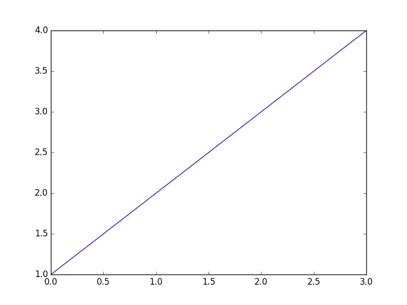
Two things to note from this plot:

  • pyplot.plot causeless our unmarried data listing to be the y-values;

  • in the absenteeism of an x-values listing, [0, 1, two, 3] was used instead.

    Note

    pyplot is commonly used abbreviated as plt , just as numpy is unremarkably abbreviated as np . The remainder of this chapter uses the abbreviated form.

    Annotation

    Enhanced interactive python interpreters such as IPython can automate some of the plotting calls for y'all. For instance, y'all can run %matplotlib in IPython, after which y'all no longer need to run plt.prove everytime when calling plt.plot . For simplicity, plt.show volition likewise be left out of the remainder of these examples.

If you pass two lists to plt.plot you and then explicitly ready the x values:

                                    >>>                                    plt                  .                  plot                  ([                  0.i                  ,                  0.2                  ,                  0.3                  ,                  0.4                  ],                  [                  ane                  ,                  two                  ,                  3                  ,                  4                  ])                

_images/mpl_basic2.png

Understandably, if you provide ii lists their lengths must lucifer:

                                >>>                                plt                .                plot                ([                0.ane                ,                0.2                ,                0.3                ,                0.4                ],                [                1                ,                2                ,                iii                ,                4                ,                five                ])                ValueError: 10 and y must have same commencement dimension              

To plot multiple curves simply call plt.plot with every bit many xy listing pairs every bit needed:

                                    >>>                                    plt                  .                  plot                  ([                  0.ane                  ,                  0.two                  ,                  0.3                  ,                  0.iv                  ],                  [                  1                  ,                  2                  ,                  3                  ,                  4                  ],                                      [0.i, 0.2, 0.3, 0.4], [1, 4, 9, 16])                

_images/mpl_basic3.png

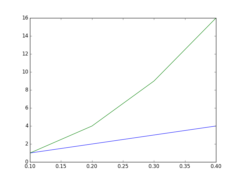
Alternaltively, more plots may be added past repeatedly calling plt.plot . The post-obit code snippet produces the aforementioned plot as the previous code example:

                                >>>                                plt                .                plot                ([                0.1                ,                0.2                ,                0.3                ,                0.4                ],                [                ane                ,                2                ,                3                ,                iv                ])                >>>                                plt                .                plot                ([                0.1                ,                0.2                ,                0.3                ,                0.4                ],                [                1                ,                4                ,                9                ,                16                ])              

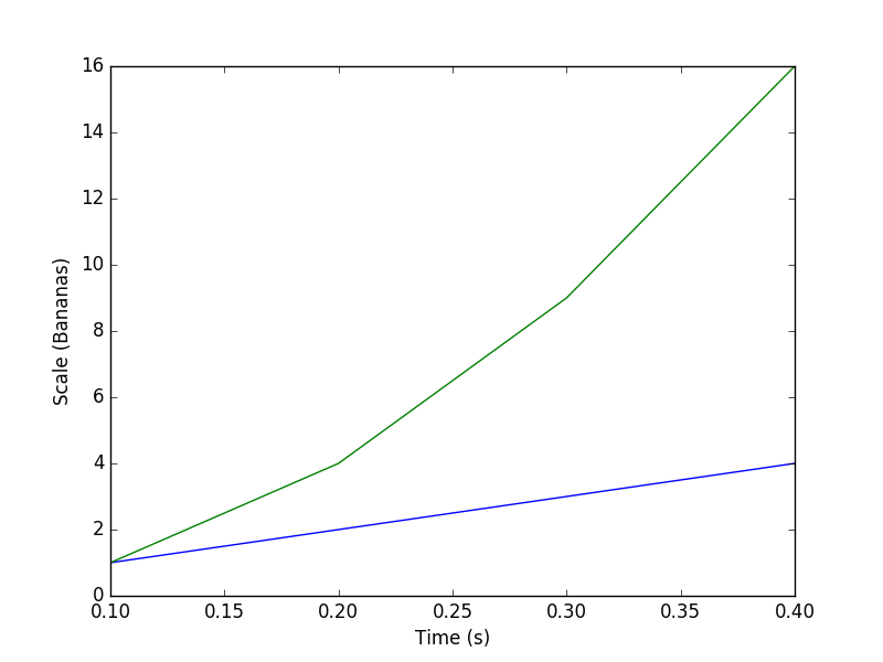
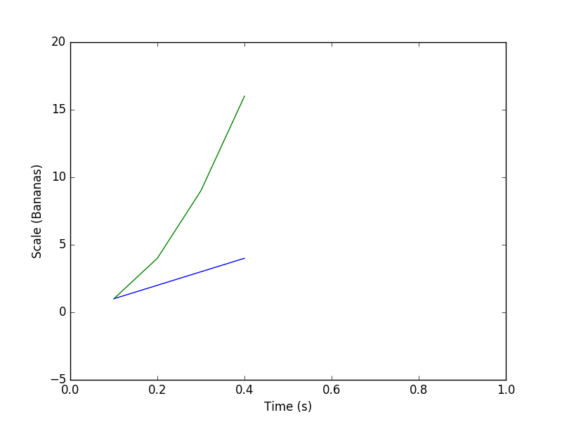
Adding information to the plot axes is straightforward to practise:

                                    >>>                                    plt                  .                  plot                  ([                  0.1                  ,                  0.2                  ,                  0.3                  ,                  0.four                  ],                  [                  ane                  ,                  2                  ,                  3                  ,                  four                  ])                  >>>                                    plt                  .                  plot                  ([                  0.1                  ,                  0.ii                  ,                  0.3                  ,                  0.four                  ],                  [                  1                  ,                  4                  ,                  9                  ,                  16                  ])                  >>>                                    plt                  .                  xlabel                  (                  "Fourth dimension (s)"                  )                  >>>                                    plt                  .                  ylabel                  (                  "Calibration (Bananas)"                  )                

_images/mpl_basic4.png

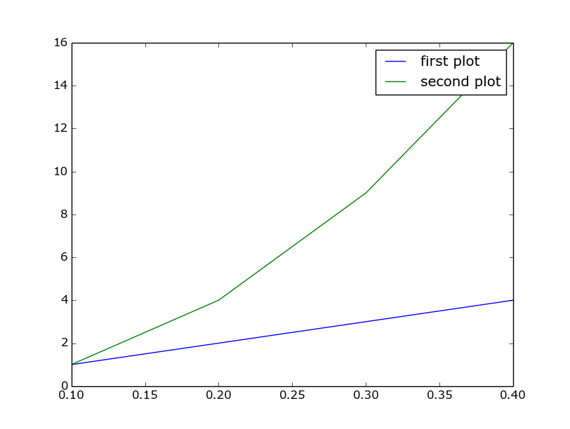
Also, adding an legend is rather simple:

                                    >>>                                    plt                  .                  plot                  ([                  0.1                  ,                  0.2                  ,                  0.3                  ,                  0.4                  ],                  [                  1                  ,                  2                  ,                  3                  ,                  4                  ],                  label                  =                  'starting time plot'                  )                  >>>                                    plt                  .                  plot                  ([                  0.one                  ,                  0.two                  ,                  0.3                  ,                  0.4                  ],                  [                  1                  ,                  4                  ,                  9                  ,                  16                  ],                  label                  =                  'second plot'                  )                  >>>                                    plt                  .                  legend                  ()                

_images/mpl_basic4c.png

And adjusting axis ranges can be done past calling plt.xlim and plt.ylim with the lower and higher limits for the corresponding axes.

                                    >>>                                    plt                  .                  plot                  ([                  0.1                  ,                  0.two                  ,                  0.iii                  ,                  0.iv                  ],                  [                  one                  ,                  2                  ,                  3                  ,                  4                  ])                  >>>                                    plt                  .                  plot                  ([                  0.1                  ,                  0.2                  ,                  0.3                  ,                  0.iv                  ],                  [                  ane                  ,                  4                  ,                  9                  ,                  16                  ])                  >>>                                    plt                  .                  xlabel                  (                  "Time (due south)"                  )                  >>>                                    plt                  .                  ylabel                  (                  "Calibration (Bananas)"                  )                  >>>                                    plt                  .                  xlim                  (                  0                  ,                  i                  )                  >>>                                    plt                  .                  ylim                  (                  -                  5                  ,                  20                  )                

_images/mpl_basic4b.png

In addition to x and y data lists, plt.plot tin can as well accept strings that define the plotting style:

                                    >>>                                    plt                  .                  plot                  ([                  0.1                  ,                  0.two                  ,                  0.three                  ,                  0.four                  ],                  [                  1                  ,                  2                  ,                  3                  ,                  4                  ],                  'rx'                  )                  >>>                                    plt                  .                  plot                  ([                  0.ane                  ,                  0.2                  ,                  0.three                  ,                  0.four                  ],                  [                  1                  ,                  4                  ,                  ix                  ,                  sixteen                  ],                  'b-.'                  )                  >>>                                    plt                  .                  xlabel                  (                  "Fourth dimension (s)"                  )                  >>>                                    plt                  .                  ylabel                  (                  "Scale (Bananas)"                  )                
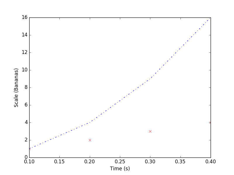
_images/mpl_basic5.png

The way strings, one per xy pair, specify color and shape: 'rx' stands for red crosses, and 'b-.' stands for blueish dash-point line. Check the documentation of pyplot.plot for the listing of colors and shapes.

Finally, plt.plot can besides, conveniently, take numpy arrays as its arguments.

More plots

While plt.plot can satisfy basic plotting needs, matplotlib provides many more plotting functions. Below nosotros effort out the plt.bar role, for plotting bar charts. The full list of plotting functions tin be plant in the the matplotlib.pyplot documentation.

Bar charts can be plotted using plt.bar , in a similar fashion to plt.plot :

                                    >>>                                    plt                  .                  bar                  (                  range                  (                  7                  ),                  [                  1                  ,                  2                  ,                  three                  ,                  4                  ,                  3                  ,                  2                  ,                  ane                  ])                

_images/mpl_bar.png

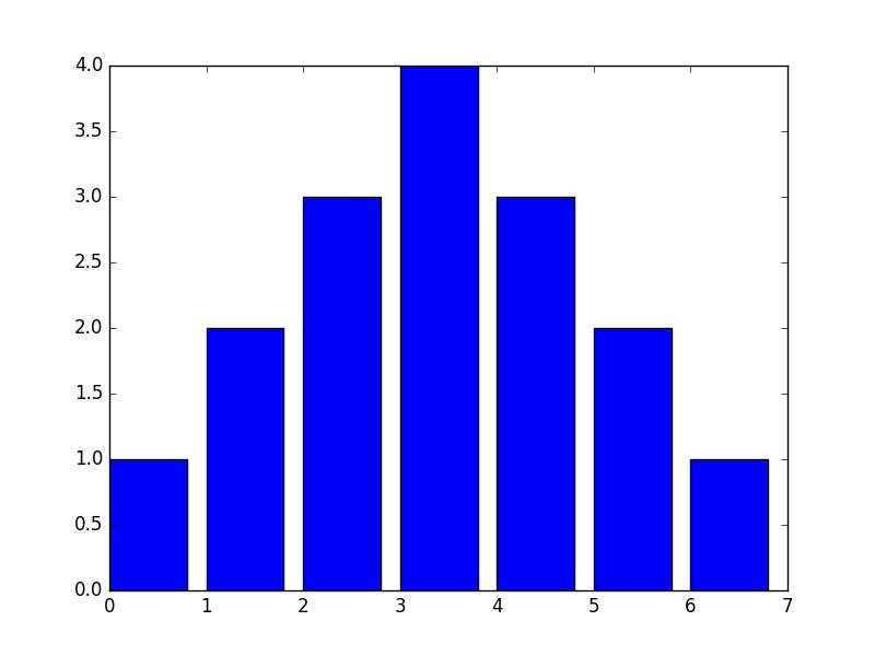
Notation, however, that contrary to plt.plot you must e'er specify x and y (which stand for, in bar nautical chart terms to the left bin edges and the bar heights). Also notation that you lot tin can only plot one nautical chart per phone call. For multiple, overlapping charts you lot'll need to telephone call plt.bar repeatedly.

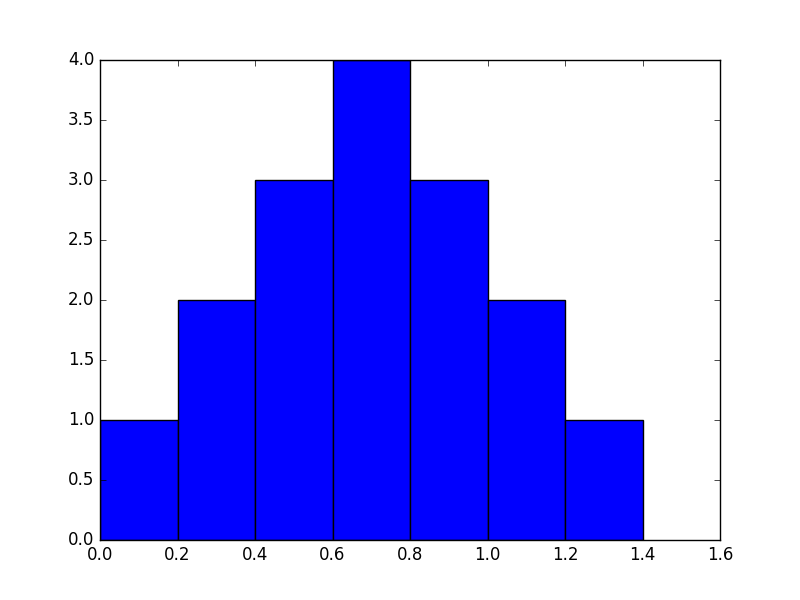
I of the optional arguments to plt.bar is width , which lets you specify the width of the bars. Its default of 0.8 might not be the nigh suited for all cases, especially when the x values are minor:

                                    >>>                                    plt                  .                  bar                  (                  numpy                  .                  arange                  (                  0.                  ,                  i.4                  ,                  .                  2                  ),                  [                  1                  ,                  2                  ,                  3                  ,                  four                  ,                  3                  ,                  2                  ,                  ane                  ])                

_images/mpl_bar2.png

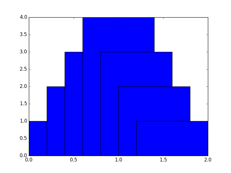
Specifying narrower confined gives us a much amend event:

                                    >>>                                    plt                  .                  bar                  (                  numpy                  .                  arange                  (                  0.                  ,                  1.4                  ,                  .                  2                  ),                  [                  1                  ,                  2                  ,                  3                  ,                  iv                  ,                  3                  ,                  2                  ,                  ane                  ],                  width                  =                  0.ii                  )                

_images/mpl_bar3.png

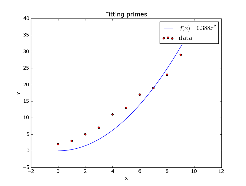
Sometimes you will want to compare a role to your measured data; for instance when y'all simply fitted a part. Of course this is possible with matplotlib. Let'due south say we fitted an quadratic function to the first 10 prime numbers, and want to check how practiced our fit matches our data.

                          1  ii  3  4  5  6  7  eight  9 x 11 12 13 14 15 16 17 eighteen 19 20 21
                                                    import                          matplotlib.pyplot                          as                          plt                          def                          found_fit                          (                          x                          ):                          render                          0.388                          *                          ten                          **                          2                          # Institute with symfit.                          x_data                          =                          list                          (                          range                          (                          10                          ))                          y_data                          =                          [                          2                          ,                          3                          ,                          5                          ,                          7                          ,                          11                          ,                          13                          ,                          17                          ,                          19                          ,                          23                          ,                          29                          ]                          x_func                          =                          np                          .                          linspace                          (                          0                          ,                          x                          ,                          50                          )                          # numpy will exercise the right thing and evaluate found_fit for all elements                          y_func                          =                          found_fit                          (                          x_func                          )                          # From here the plotting starts                          plt                          .                          scatter                          (                          x_data                          ,                          y_data                          ,                          c                          =                          'r'                          ,                          label                          =                          'data'                          )                          plt                          .                          plot                          (                          x_func                          ,                          y_func                          ,                          label                          =                          '$f(x) = 0.388 x^two$'                          )                          plt                          .                          xlabel                          (                          'x'                          )                          plt                          .                          ylabel                          (                          'y'                          )                          plt                          .                          title                          (                          'Fitting primes'                          )                          plt                          .                          legend                          ()                          plt                          .                          show                          ()                        

We fabricated the scatter plot blood-red by passing information technology the keyword statement c='r' ; c stands for colour, r for red. In improver, the label we gave to the plot statement is in LaTeX format, making it very pretty indeed. Information technology's not a great fit, simply that's besides the point here.

_images/mpl_scatter.png

Interactivity and saving to file

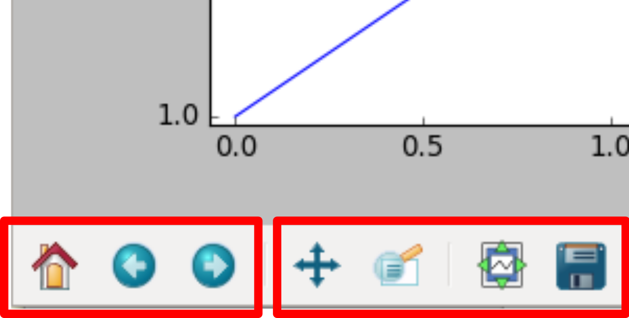
If yous tried out the previous examples using a Python/IPython console yous probably got for each plot an interactive window. Through the four rightmost buttons in this window you can do a number of actions:

  • Pan around the plot expanse;
  • Zoom in and out;
  • Access interactive plot size control;
  • Save to file.

The three leftmost buttons volition allow you to navigate between dissimilar plot views, subsequently zooming/panning.

_images/mpl_buttons2.png

As explained higher up, saving to file tin be easily washed from the interactive plot window. Nonetheless, the demand might arise to take your script write a plot directly every bit an image, and non bring upward whatever interactive window. This is easily done by calling plt.savefig :

                                    >>>                                    plt                  .                  plot                  ([                  0.ane                  ,                  0.2                  ,                  0.three                  ,                  0.4                  ],                  [                  1                  ,                  two                  ,                  iii                  ,                  4                  ],                  'rx'                  )                  >>>                                    plt                  .                  plot                  ([                  0.1                  ,                  0.2                  ,                  0.3                  ,                  0.4                  ],                  [                  1                  ,                  4                  ,                  nine                  ,                  xvi                  ],                  'b-.'                  )                  >>>                                    plt                  .                  xlabel                  (                  "Time (s)"                  )                  >>>                                    plt                  .                  ylabel                  (                  "Scale (Bananas)"                  )                  >>>                                    plt                  .                  savefig                  (                  'the_best_plot.pdf'                  )                

Notation

When saving a plot, y'all'll want to choose a vector format (either pdf, ps, eps, or svg). These are resolution-contained formats and will yield the all-time quality, even if printed at very large sizes. Saving as png should be avoided, and saving as jpg should be avoided even more.

Multiple figures

With this background out of the way, we can movement on to some more advanced matplotlib use. It is also possible to use it in an object-oriented manner, which allows for more than separation between several plots and figures. Let's say we have 2 sets of data we desire to plot next to eachother, rather than in the same figure. Matplotlib has several layers of organisation: beginning, there'southward an Figure object, which basically is the window your plot is fatigued in. On summit of that, there are Axes objects, which are your divide graphs. It is perfectly possible to have multiple (or no) Axes in one Figure. We'll explain the add_subplot method a fleck later. For now, information technology only creates an Centrality example.

                            1  2  3  four  five  half dozen  seven  8  nine x xi 12 13
                                                        import                            matplotlib.pyplot                            as                            plt                            x_data                            =                            [                            0.1                            ,                            0.2                            ,                            0.3                            ,                            0.4                            ]                            y_data                            =                            [                            1                            ,                            two                            ,                            3                            ,                            4                            ]                            fig                            =                            plt                            .                            figure                            ()                            ax                            =                            fig                            .                            add_subplot                            (                            1                            ,                            i                            ,                            1                            )                            ax                            .                            plot                            ([                            0.1                            ,                            0.2                            ,                            0.iii                            ,                            0.four                            ],                            [                            1                            ,                            2                            ,                            three                            ,                            4                            ])                            ax                            .                            plot                            ([                            0.1                            ,                            0.2                            ,                            0.3                            ,                            0.4                            ],                            [                            i                            ,                            iv                            ,                            nine                            ,                            16                            ])                            ax                            .                            set_xlabel                            (                            'Time (s)'                            )                            ax                            .                            set_ylabel                            (                            'Scale (Bananas)'                            )                            plt                            .                            show                            ()                          

_images/mpl_basic4.png

This example too neatly highlights one of Matplotlib'south shortcomings: the API is highly inconsistent. Where we could do xlabel() before, we now need to practise set_xlabel() . In addition, nosotros tin can't show the figures one by one (i.east. fig.show() ); instead nosotros tin only show them all at the same time with plt.prove() .

Now, we desire to make multiple plots adjacent to each other. We exercise that by calling plot on 2 different axes:

                            1  2  3  4  5  6  7  8  9 x 11 12 13 fourteen 15 16 17 eighteen 19 xx 21
                                                        x_data1                            =                            [                            0.1                            ,                            0.2                            ,                            0.3                            ,                            0.4                            ]                            y_data1                            =                            [                            one                            ,                            2                            ,                            3                            ,                            four                            ]                            x_data2                            =                            [                            0.1                            ,                            0.two                            ,                            0.iii                            ,                            0.4                            ]                            y_data2                            =                            [                            ane                            ,                            4                            ,                            ix                            ,                            16                            ]                            fig                            =                            plt                            .                            effigy                            ()                            ax1                            =                            fig                            .                            add_subplot                            (                            i                            ,                            2                            ,                            1                            )                            ax2                            =                            fig                            .                            add_subplot                            (                            1                            ,                            2                            ,                            2                            )                            ax1                            .                            plot                            (                            x_data1                            ,                            y_data1                            ,                            label                            =                            'data 1'                            )                            ax2                            .                            plot                            (                            x_data2                            ,                            y_data2                            ,                            label                            =                            'data ii'                            )                            ax1                            .                            set_xlabel                            (                            'Time (s)'                            )                            ax1                            .                            set_ylabel                            (                            'Scale (Bananas)'                            )                            ax1                            .                            set_title                            (                            'commencement information gear up'                            )                            ax1                            .                            fable                            ()                            ax2                            .                            set_xlabel                            (                            'Fourth dimension (s)'                            )                            ax2                            .                            set_ylabel                            (                            'Scale (Bananas)'                            )                            ax2                            .                            set_title                            (                            '2d information set'                            )                            ax2                            .                            legend                            ()                            plt                            .                            show                            ()                          

_images/mpl_oop1.png

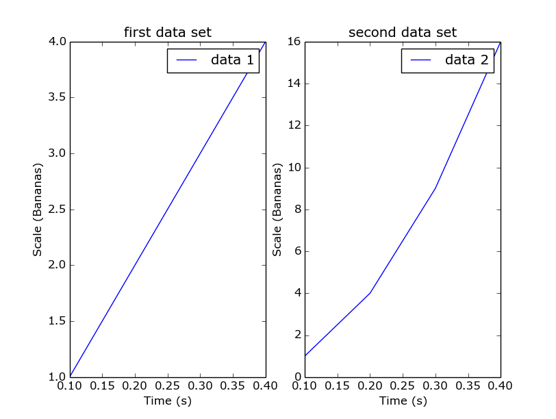
The add_subplot method returns an Centrality instance and takes three arguments: the start is the number of rows to create; the second is the number of columns; and the last is which plot number we add right now. So in mutual usage you will need to phone call add_subplot one time for every axis you want to brand with the aforementioned get-go two arguments. What would happen if you first inquire for one row and two columns, and for two rows and one column in the next phone call?

Exercises

  1. Plot a dashed line.
  2. Search the matplotlib documentation, and plot a line with plotmarkers on all it'due south datapoints. You can exercise this with simply one phone call to plt.plot .